LimeADPD I/Q - DPD with I/Q Imbalance Mitigation

Transmitter I/Q imbalance

Complex-valued signal x(t), exposed to the source of frequency-independent I/Q imbalance, results to the signal y(t):

\[y(t)=\eta_1 x(t) + \eta_2 x^*(t)\]

\[\eta_1=\cos \frac{\phi}{2} + j \epsilon \sin\frac{\phi}{2}\]

\[\eta_2= \epsilon \cos\frac{\phi}{2} - j \sin\frac{\phi}{2}\]

The parameters ε and φ represent the amplitude and phase imbalance terms. For wideband signals, I/Q imbalance manifests frequency-dependent behavior caused by analogue components in I and Q modulator paths.

LimeADPD I/Q method is used for joint PA linearization and RF transmitter I/Q imbalance mitigation. It is designed for implementation in software-defined radio (SDR) base stations (BS).

LimeADPD I/Q Indirect Learning Architecture

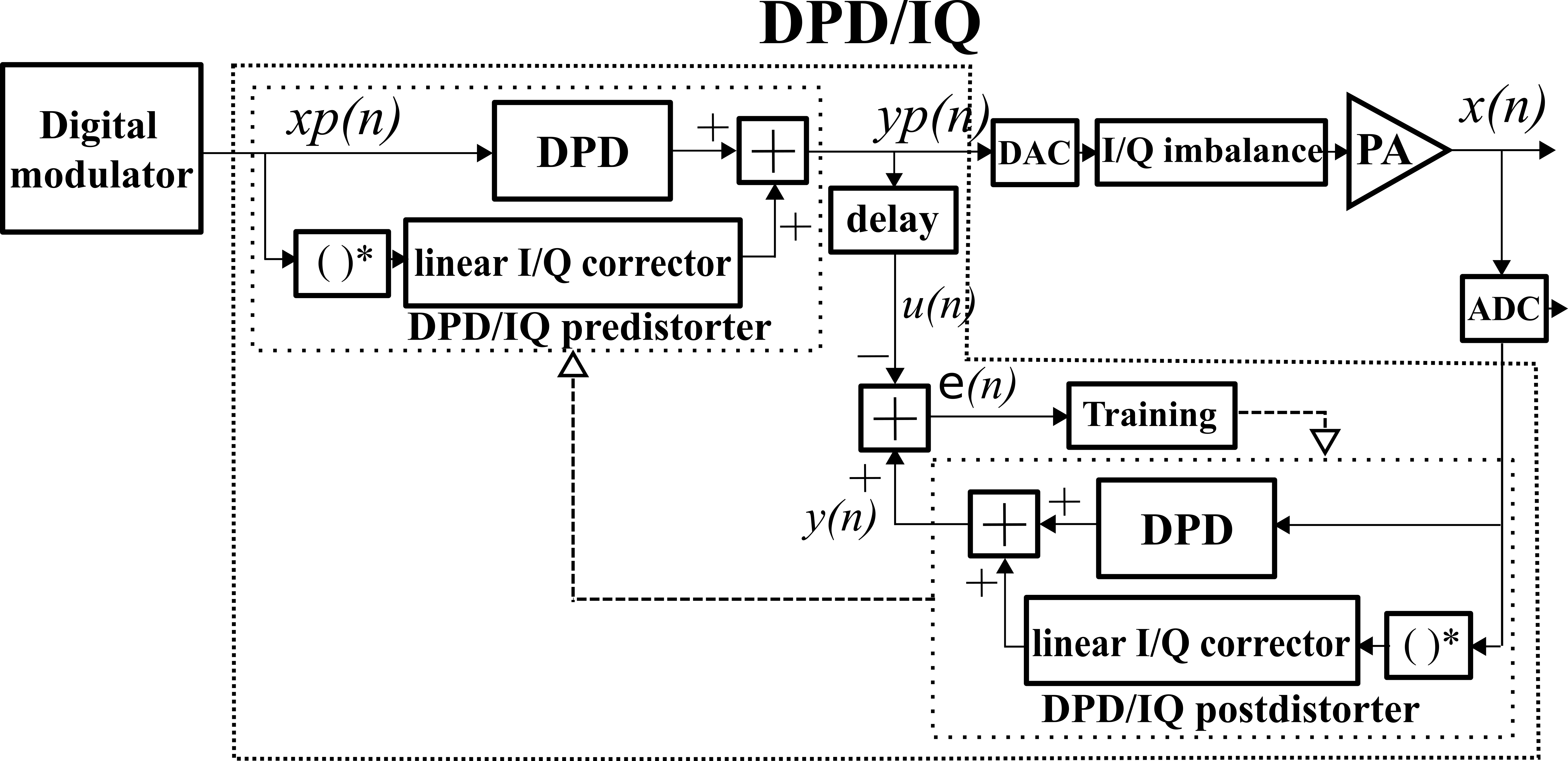
The modification of LimeADPD which performs joint PA nonlinearity minimization and I/Q imbalance mitigation is given in Figure 2.

Pre-distorter and post-distorter blocks are divided into Memory Polynomial (MP) based non-conjugate and linear conjugate sub-blocks, as presented in Figure 2. The pre-distorter MP non-conjugate part (named with DPD in the Figure 2) takes at input signal xp(n):

\[xp(n)=xp_I(n)+jxp_Q(n)\]

and it is dedicated to minimization of PA and transmitter nonlinearity effects. The linear conjugate part, denoted as I/Q corrector, takes at input the complex-conjugated signal xp*(t):

\[xp^*(n)=xp_I(n)-jxp_Q(n)\]

and is introduced to suppress the effects of transmitter’s I/Q imbalance.

Figure 2: Indirect learning architecture for I/Q image rejection and PA linearization

Complex Valued Memory Polynomial

For a given complex input:

\[x(n)=x_I(n)+jx_Q(n)\]

and conjugated complex input signal:

\[x^*(n)=x_I(n)-jx_Q(n)\]

LimeADPD I/Q model produces complex output:

\[y(n)=y_I(n)+jy_Q(n)\]

\[y(n)=\sum_{i_1=0}^{N_1} \sum_{j_1=0}^{M_1} g_{i_1j_1} x(n-i_1)e(n-i_1)^{j_1} + \sum_{i_2=0}^{N_2} \ h_{i_2} x^*(n-i_2)\]

where:

\[g_{i_1j_1}=a_{i_1j_1}+jb_{i_1j_1}\]

\[h_{i_2}=c_{i_2}+jd_{i_2}\]

are the polynomial coefficients while e(n) is the squared envelope of the input:

\[e(n)=x_I(n)^2+x_Q(n)^2\]

In the above equations, parameter N₁represents the DPD memory length and M₁is the nonlinearity order. The I/Q corrector block is modeled by linear FIR filter block with length N₂.

The advantage of LimeADPD I/Q is low complexity in terms of reduced number of complex valued coefficients.

LimeADPD I/Q Equations

Based on discussions given in previous sections and using signal notations of Figure 2, the ADPD I/Q pre-distorter implements the following equations:

\[yp(n)=\sum_{i_1=0}^{N_1} \sum_{j_1=0}^{M_1} g_{i_1j_1} xp(n-i_1)ep(n-i_1)^{j_1} + \sum_{i_2=0}^{N_2} \ h_{i_2} xp^*(n-i_2)\]

\[xp(n)=xp_I(n)+jxp_Q(n)\]

\[xp^*(n)=xp_I(n)-jxp_Q(n)\]

\[ep(n)=xp_I(n)^2+xp_Q(n)^2\]

while the post-distorter does similar:

\[y(n)=\sum_{i_1=0}^{N_1} \sum_{j_1=0}^{M_1} g_{i_1j_1} x(n-i_1)e(n-i_1)^{j_1} + \sum_{i_2=0}^{N_2} \ h_{i_2} x^*(n-i_2)\]

\[x(n)=x_I(n)+jx_Q(n)\]

\[x^*(n)=x_I(n)-jx_Q(n)\]

\[e(n)=x_I(n)^2+x_Q(n)^2\]

Note that the pre-distorter and post-distorter share the same set of complex coefficients g and h. Delay line is given by:

\[u(n)=yp(n-nd)\]

LimeADPD I/Q Training Algorithm

The LimeADPD I/Q training algorithm alters complex valued memory polynomial coefficients in order to minimize the difference between PA input yp(n) and y(n). The instantaneous error shown is calculated as:

\[\epsilon(n)=\sqrt{(u_I(n)-y_I(n))^2+(u_Q(n)-y_Q(n))^2}\]

Training is based on minimising Recursive Least Square E(n) error:

\[E(n)=\frac{1}{2}\sum_{m=0}^{n} \lambda^{n-m} \epsilon(m)^2, \lambda<1\]

by solving linear system of equations:

\[\frac{\partial E(n)}{\partial a_{i_1j_1}}=0; \frac{\partial E(n)}{\partial b_{i_1j_1}}=0; \frac{\partial E(n)}{\partial c_{i_2}}=0; \frac{\partial E(n)}{\partial d_{i_2}}=0;\]

\[i_1=0,1,...,N_1; j_1=0,1,...,M_1; i_2=0,1,...,N_2;\]

Following RLS algorithm, after every training step, the system of equations is solved. Lime ADPD I/Q involves LU decomposition for equation solving method.